
An LC oscillator is a circuit which we can use to transform a direct current (DC) supply voltage into an alternating current (AC) output waveform. This output can exhibit various types of waveform shapes and frequencies which might range from complex forms to simple pure sine waves depending on the specific application requirements.
These oscillators are widely used in test equipment (like function generators) and may generate a wide range of waveforms, including sinusoidal, square, sawtooth, triangular, and sequences of repeating pulses with constant or variable width. You will find that LC oscillators are especially popular in radio-frequency (RF) circuits due to their excellent phase noise performance and simplicity of design.
Basics of Oscillators
At its most basic, an oscillator is an amplifier that uses positive feedback, sometimes known as regenerative feedback, to reinforce the input signal in phase. One big difficulty in electrical design happens to be regulating the inclination of amplifiers to oscillate while on the other hand ensuring that oscillators always maintain a steady oscillation.
One feature of oscillators is that they function by compensating for losses in energy in their feedback resonant circuit which is usually made up of inductors, capacitors, or a combination thereof.
They basically create oscillations by introducing DC energy into this resonant circuit at the appropriate frequency. In simple terms, an oscillator functions as a positive feedback amplifier, and provides an output frequency without the requirement for an external AC input signal.
Essential Characteristics of Oscillators
To be eligible to serve as an oscillator, a circuit must meet three essential criteria:
- Amplification: There has to be a signal amplification device in the circuit.
- Positive Feedback: In order to maintain oscillation, the circuit must use positive feedback.
- Frequency-Determining Network: There needs to be a feedback network which establishes the oscillation frequency.
To begin its oscillations, an oscillator generally uses a small-signal feedback amplifier with an open-loop gain of about equal to or slightly larger than unity. In order to ensure an uninterrupted oscillation, the average loop gain of the oscillator circuit must be stable at unity. To guarantee this, it requires the addition of reactive components together with an active amplifying device, which could be an operational amplifier (Op-Amp) or bipolar junction transistor (BJT).
Oscillator circuits are actually not like ordinary amplifier circuits, because they have no need for an external AC signal to function, instead they are able to simply transform the supplied DC energy into AC energy at the appropriate frequency, allowing them to generate self-sustaining periodic output waveforms, usually at a single sinusoidal frequency.
Understanding a Basic Oscillator Feedback Circuit

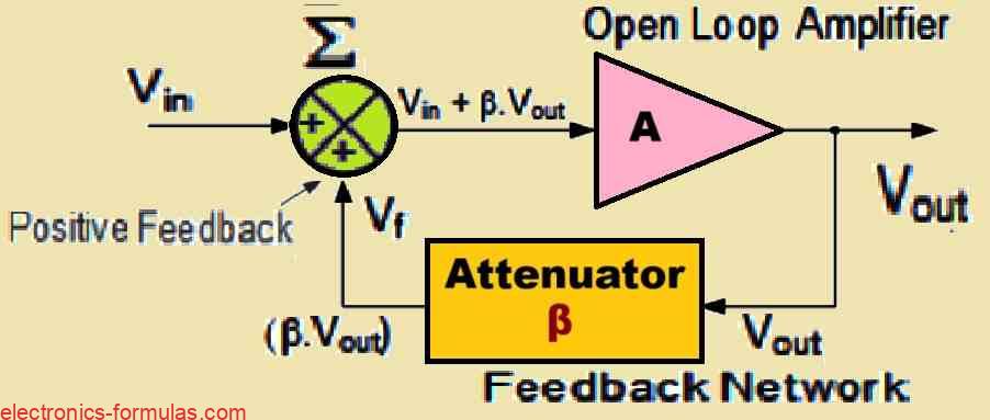
In the above diagram the “β” represents a feedback fraction.
Calculating Gain of the Oscillator Circuit Without Feedback
Gain, A = VOUT/VIN (where A is the open loop voltage gain)
∴ VOUT = A * VIN
Calculating Gain of the Oscillator Circuit With Feedback
A(VIN + βVOUT) = VOUT, where β is the feedback fraction
A * VIN + A * βVOUT = VOUT where Aβ equals the voltage loop gain
A * VIN = VOUT (1 – Aβ), where 1 – Aβ is equal to positive feedback factor
∴ VOUT/VIN = Gv = A/(1 – Aβ), where Gv equals the closed loop voltage gain.
Oscillators are specialized electronic circuits which are designed to produce a continuous voltage output waveform at a specified frequency. And they typically incorporate inductors, capacitors, or resistors to create a frequency-selective resonant circuit. Basically you may find that an oscillator circuit functions similar to a passive band-pass filter selectively allowing just the required frequency to pass while attenuating others. Furthermore a crucial feedback network is incorporated into the design to assure that the waveforms have continued non-stop oscillations, hence improving the oscillator’s overall performance and stability.
The feedback network is critical to the oscillation process because it “feeds” a tiny fraction of the output signal back to the input side, which is required for the circuit to oscillate continuously. It is extremely important that the quantity of positive feedback given is adequate to compensate for any losses in the circuit, allowing the output waveform to oscillate continuously for an unlimited duration.
Actually the feedback network functions just like an attenuation circuit, characterized by a voltage gain of less than one (β < 1). You will find that oscillations take place as soon as the amplifier gain (A) and feedback factor (β) reach unity (Aβ > 1), and then once oscillations start to occur, the above product Aβ stabilizes back to unity (Aβ = 1), guaranteeing that the oscillation process goes on continuously.
The frequency of the LC oscillator is controlled by incorporating a precisely calibrated circuit which is actually a resonant inductive-capacitive (LC) circuit. We call this output frequency produced through this inductive-capacitive (LC) circuit setup as the “oscillation frequency”. By incorporating a reactive network into the feedback mechanism of the oscillator, the phase angle associated with this feedback can change with respect to the variations in frequency, and this phenomenon is termed as the “Phase-shift”.
Types of Oscillators
We can fundamentally classify oscillators into two distinct categories:
1. Sinusoidal Oscillators: The sinusoidal or harmonic oscillators operate by using tuned feedback involving either RC network or LC network configurations. What separates them is that they are able to generate a perfectly sinusoidal waveform over time that has a very stable frequency and amplitude.
2. Non Sinusoidal Oscillators –These type of Oscillators (also known as relaxation oscillators) are able to create some waveforms that are not in the sinusoidal shape. When these oscillators change between each of their stable states, waveforms as sawtooth, triangle, and square wave are produced. These waveforms, which help illustrate the complexities in chaotic non-sinusoidal oscillation behavior, each have their own unique signature form and characteristics.
Understanding Resonance in Oscillator Circuits
When we apply a constant voltage that varies with frequency to a circuit consisting of an inductor, capacitor, and resistor, the resulting reactance associated with the capacitor and resistor, as well as the inductor and resistor, causes changes in both the amplitude and phase of the output signal with respect to the input. This phenomena is caused by the distinct reactance characteristics of the circuit’s components.
Now if we increase the applied frequencies of the supply then the capacitor behaves in such a way that its reactance drops dramatically thus operating as a short circuit. But In contrast the inductor’s reactance increases dramatically, just like an open circuit. But if we reduce the frequencies, however, the situation is reversed, now the capacitor’s reactance behaves similarly to an open circuit while on the other hand the inductor’s reactance behaves just like a short circuit.
In the middle of these two frequency extreme limits, the interaction of the inductor and capacitor results in the creation of a “tuned” or “resonant” circuit. The precise arrangement is specified by the particular Resonant Frequency, represented by the symbol (̒fr), where the inductive and capacitive reactances perfectly cancel out one another by balancing each other out. Now, the only element in the circuit remaining to resist the passage of current is the resistive component or the resistor, which simply means that there cannot be any phase shift, which in turn means that the current and voltage are exactly in phase. Please take a look at the circuit below for proper understanding.
Understanding Basic LC Oscillator Tank Circuit

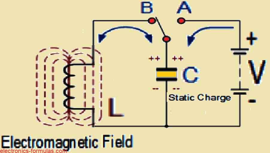
The two main parts of the circuit are an inductive coil (L) and a capacitor (C). The job of the capacitor is to store energy as an electric field which causes a potential, or static voltage, to be created across its plates. However the purpose of the inductive coil is to store energy as an electromagnetic field. Next, we turn ON the switch to position A to connect the capacitor to the DC supply voltage, or V, and start its charging process. Then subsequently we change the position of the switch to position B to finish the circuit operation when the capacitor has reached its full charge.
Now that the charged capacitor and the inductive coil are linked in parallel, the capacitor may start to discharge through the coil. The current passing through the coil starts to increase as this process progresses, while the voltage across the capacitor C starts to drop.
This increase in current creates an electromagnetic field around the coil, which acts to restrict the passage of current. After the capacitor (C) is completely drained, the energy it contained in the form of an electrostatic field is transferred to the inductive coil (L) and stored there as an electromagnetic field around the coil’s windings.
Now because there is no external voltage in the circuit to support the current within the coil, the current begins to drop as the electromagnetic field collapses. During this phase the coil experiences the induction of a reverse electromotive force (emf) which may be expressed as e = −L (dt/di) and this keeps the current flowing in the same direction.
Due to the induced emf, the capacitor C begins to charge with current but this time the polarity of the charge gets totally reversed. This charging process keeps on happening until the coil’s electromagnetic field entirely collapses and the current drops to zero.
Now that the circuit has received the energy that was first introduced by the switch, the electrostatic voltage potential between the capacitor’s plates is once again present, however, this potential is now the opposite of what it was in the beginning. At this moment the cycle repeats itself as the capacitor starts to discharge through the coil once more.
So now, as the energy oscillates back and forth across the capacitor and the inductor, the polarity of the voltage alternates, which produces an alternating current (AC) type sinusoidal waveform for both voltage and current.
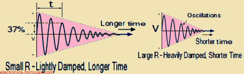
This alternate cycle of repetition establishes the foundation for the tank circuit of an LC oscillator, which simply means that this oscillation in which energy alternates between states might potentially last forever. But the truth is that there are never ideal circumstances, because some energy losses will take place each time energy is sent from the capacitor C to the inductor L and then back from L to C, and ultimately these losses will cause the oscillations to steadily decrease until they ultimately hit zero.
In the ideal world the energy that is always oscillating between the capacitor C and the inductor L would never stop if it hadn’t been for the circuit’s intrinsic energy losses. These losses show up as the dissipation of electrical energy in several ways such as the inductor’s coil’s actual resistance or direct current (DC), the capacitor’s dielectric material, and the circuit’s radiation. Because of these losses, the oscillations will gradually decrease until they vanish entirely which finally stops the process altogether.
In a practical real world LC circuit, the amplitude of the oscillatory voltage will decrease with each half cycle of oscillation eventually decaying to almost zero. These type of oscillations are hence referred to as “damped.” The quality of the circuit, also known as the Q-factor, affects how much damping occurs. Although a lower Q-factor results in more energy dissipation and more noticeable damping of the oscillations, a higher Q-factor suggests less energy loss and therefore reduced damping.
What is Damped Oscillations

We can determine the frequency of the oscillating voltage in the LC tank circuit by appropriately selecting the inductance and capacitance values of the tank circuit. In order to achieve resonance in the tank circuit, we must remember that there must be a precise frequency at which the inductive reactance (XL) and capacitive reactance (XC) are equal. As soon as these two reactances become equal to each other (XL=XC), they essentially cancel each other out and then only we have the DC resistance in the circuit to prevent current flow.
To better illustrate this idea we can consider superimposing the curves for the capacitive reactance of the capacitor and the inductive reactance of the inductor, so that they line up along the same frequency axis. Then we are quickly able to point out the resonance frequency (fr or 𝜏r) at the point where the curves cross each other. This junction point is important because it tells us and indicates the specific situation at which resonance is reached in the tank circuit.
Understanding the Resonance Frequency

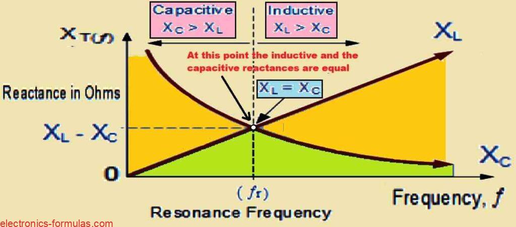
Referring to the above diagram, here fr will be in Hertz, the L will be in Henries and C will be in Farads.
So, now we can express the frequency at which this resonance will take place through the following equations:
XL = 2πfL and XC = 1/2πfC
when resonance happens, at that point, XL = XC
∴ 2πfL = 1/2πfC
2πf2L = 1/2πC
∴ f2 = 1/(2π)2LC
∴ f = √1/√[(2π)2LC]
Now it is possible for us to make the above result even more simpler and obtain the following finalized equation for calculating the Resonant Frequency fr in any tuned LC circuit:
Formula for the Resonant Frequency of an LC Oscillator
fr = 1/2π√LC
- Where:
- L represents the Inductance in Henries
- C represents the Capacitance in Farads
- fr represents the Output Frequency in Hertz
From the above equation we realize that if any one of the parameters L or C are decreased, then the frequency increases. We can generally express this output frequency using the abbreviation fr to indicate the “resonant frequency”.
To keep the oscillations going in an LC tank circuit, we have to replace all the energy lost in each oscillation and also maintain the amplitude of these oscillations at a constant level. The amount of energy replaced must therefore be equal to the energy lost during each cycle.
In an LC tank circuit, we must make sure that all energy lost during each oscillation must be restored and the oscillations amplitude kept constant in order to keep the oscillations running. As a result it is important that the magnitude of energy restored should match the quantity of energy lost throughout each cycle.
However if the amount of energy replaced is excessive, that would cause the amplitude to climb until the supply rails clip. On the other hand, if the quantity of energy restored was too little, that would cause the oscillations to die out, because then the amplitude would ultimately tend to drop to zero.
That said, replacing this lost energy could be actually accomplished most simply by amplifying a portion of the output from the LC tank circuit and then feeding it back into the LC circuit. To implement we could simply utilize a voltage amplifier built using an op-amp, FET, or bipolar transistor as its active device. But we have also remember that if the above feedback amplifier’s loop gain is too high, then the waveform would be distorted, and if it is too small would cause the intended oscillation to decay to zero.
The total amount of energy through the feedback loop being sent to the LC network has to be precisely regulated in order to achieve a continuous oscillation. If in case the amplitude of the oscillations attempts to deviate either up or down from a reference voltage, then it may become imperative for us to include some sort of automated amplitude or gain control in the circuit.
In order to sustain a constant oscillation, we have to ensure that the total gain of the circuit is equal to 1 or unity. If suppose the gain is too small then the oscillations will simply fail to start-up or decay towards zero, and if the gain is too high, then the supply rails will start clipping the oscillation amplitude, giving rise to distortions. Please now take a look at the circuit below.
Analyzing a Basic Transistorized LC Oscillator Circuit

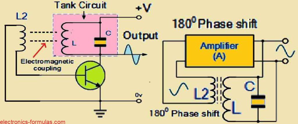
As can be seen in the above diagram, we have used an Bipolar Transistor as an amplifier in an LC oscillator which includes a tuned LC tank circuit that acts as the load for the transistor. You can also see that there’s one more coil, called L2, connected between the base and emitter of the transistor. The electromagnetic field from coil L2 interacts with the electromagnetic field of coil L; which means that the two coil start working with mutual inductance.
This mutual inductance causes the changing current in one coil to create a voltage in the other coil through electromagnetic induction. As the oscillations happen in the tuned circuit, energy moves from coil L to coil L2, which causes the generation of a voltage at the same frequency as the oscillations. Then this voltage is fed back to the transistor, helping it to amplify the signal.
We can easily adjust this feedback amount by modifying the distance between the two coils, or by adjusting how closely the two coils, L and L2, are connected. When the circuit is oscillating, its impedance behaves like a resistor, and the voltages at the collector and base of the transistor are 180 degrees out of phase. In order to keep the oscillations going non-stop (called frequency stability), it is important that the voltage in the tuned circuit must be in-phase with the oscillations.
So, to achieve this we need to introduce another 180-degree phase shift in the feedback from the collector to the base. To do this we have to make sure that the winding direction of the L2 coil is set correctly with respect to the coil L or by using a phase shift network between the BJT amplifier’s output and input.
Because of the phase shift involved we mostly call this type of LC Oscillator as the “Sinusoidal Oscillator” or a “Harmonic Oscillator”. These LC oscillators have the capability to generate high frequency sine waves and are commonly applied in devices involving radio frequency (RF) in which the amplifier section is built using a BJT or an FET.
You will see that there are actually various types of harmonic oscillators because there are many ways you can create an LC filter network and amplifier. Some common types of these harmonic oscillators include the Hartley LC Oscillator, Colpitts LC Oscillator, Armstrong Oscillator, and Clapp Oscillator.
Solving an LC oscillator Circuit Problem
Let’s consider an inductance coil having an inductance value of 150mH and a capacitor having a capacitance value of 25pF. These two components are hooked up with each other in parallel to create an oscillator circuit with an LC tank circuit. We want to calculate the frequency of oscillation of this LC oscillator circuit, let’s see how we can do it.
- We have the following Given Values:
- Inductance, L = 150 mH = 150 * 10-3 = 0.150 H
- Capacitance, C = 25 pF = 25 * 10-12 F
- Our Frequency Formula is:
f = 1 / (2π√(LC)) - First we will solve the LC calculations:
LC = 0.150 * 25 * 10-12 = 3.75 * 10-12 - Now let us solve the √(LC):
√(LC) = √(3.75 * 10-12) ≈ 0.00000193649 - Calculate 2π√(LC):
2π(0.00000193649) ≈ 0.00001216732 - Now let us Calculate the Frequency f:
f ≈ 1/(0.00001216732) ≈ 82187.36 Hz - Final Result for the frequency of oscillation is:
f ≈ 82.18 kHz
Now, you can try this, in the above calculations if you decrease the value of either the capacitance C or the inductance L, that will cause the final frequency of oscillation result of the LC tank circuit to increase.
Conclusions
From the above discussions we understand that first and foremost for the oscillations to be working and sustained, it is important that we include a reactive component in the oscillator circuit. This reactive component must be either an inductor (often denoted as L) or a capacitor (referred to as C), in addition to the obvious presence of a DC power source. Now if you test a simple inductor-capacitor circuit, you may observe that oscillations have a tendency to become damped over time, which is a phenomenon that arises due to the inherent losses across the components and the overall circuit. Therefore it becomes critically important for us to implement the voltage amplification stage, so that it becomes possible to counteract these losses and achieve a positive gain.
Furthermore we must keep in mind that the total gain of the amplifier has to be bigger than the value 1, which is often known as unity.
To guarantee sustained oscillations, we have to specifically apply a feedback which is simply a portion of the output voltage, into the tuned circuit. This feedback being provided needs to have the proper magnitude as well as precisely in phase (0°) with the original signal.
It is very important to remember that oscillations can only occur when we offer positive feedback, that supports in the process of self-regeneration of the oscillations.
Lastly, we need to be very careful regarding the total phase shift of the oscillator circuit. It is critical that this phase shift is either zero or 360 degrees, mainly because this guarantees that the output signal from the feedback network continues to be in phase with the input signal. This exact alignment is required for the oscillation process to operate effectively and sustainably.
References: LC circuit