Calculating Series RLC Resonance Circuit

Here we will explore how circuits that contain resistors (R), inductors (L), and capacitors (C) respond to different frequencies.

These circuits, called resonant circuits, behave differently depending on the frequency of the signal running through them. In this tutorial, we'll focus on a specific type called a series resonant circuit.

We'll also learn how to calculate two important frequencies: the resonant frequency and the cut-off frequencies.

Impact of Frequency on Series RLC Circuits

We've looked at series RLC circuits with a constant frequency AC source. We also saw, how phasors can combine multiple sinusoidal signals of the same frequency. But, what happens if the applied voltage has a fixed amplitude but varying frequency?

How do the inductor and capacitor, with their reactive properties, respond to this change?

In a series RLC circuit there's a specific frequency where the inductive reactance (X_L) cancels out the capacitive reactance (X_C), making X_L = X_C. This frequency is called the circuit's resonant frequency (fr).

Series resonance is crucial in electronics. It creates highly selective circuits, like those used for tuning radio and television channels, filtering AC power, or reducing noise.

Let's now analyze a simple series RLC circuit to understand this concept better.

Series RLC Circuit

To understand how frequency affects these circuits, let's revisit some key features of series RLC circuits.

• Inductive Reactance: X_L = 2πfL = ωL
• Capacitive Reactance: X_C = 1 / 2πfC = 1 / ωC
• When X_L is higher than X_C, the circuit will be inductive.
• Conversely, if X_C is higher than X_L, then the circuit will be capacitive.
• The total reactance of a circuit can be calculated using the formula:
• X_T = X_L - X_C or X_C - X_L
• The total impedance of a circuit can be calculated using the formula:
• Z = √(R² + X²_T)
• = R +jX

Inductive Reactance and Frequency: A Direct Relationship

The formula for inductive reactance (XL) shows us a clear connection: if we increase either the frequency of the current or the inductance itself, the overall inductive reactance also increases.

This makes sense because inductors resist changes in current.

Here's the key takeaway:

• Higher Frequencies, Higher Reactance: As the frequency approaches infinity, the inductive reactance climbs towards infinity as well. At this point, the inductor behaves almost like an open circuit, significantly hindering current flow.
• Lower Frequencies, Lower Reactance: On the other hand, when the frequency approaches zero (DC), the inductive reactance drops to zero. In this scenario, the inductor acts more like a short circuit, allowing current to flow freely.

This relationship between frequency and inductive reactance is perfectly captured by the curve as shown below.

Frequency Dependence of Inductive Reactance

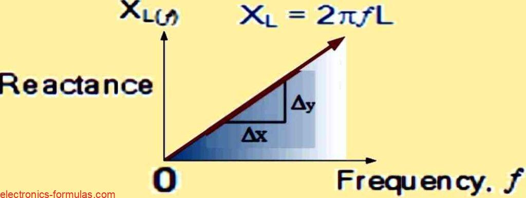
The graph depicting inductive reactance (XL) versus frequency (f) exhibits a linear characteristic. This signifies a direct proportionality between XL and f, meaning the inductive reactance of an inductor increases linearly as the applied AC current's frequency increases.

The capacitive reactance formula behaves inversely compared to inductive reactance.

In capacitors, increasing either the frequency (f) or the capacitance (C) will actually decrease the overall capacitive reactance (Xc). This is opposite to inductors where reactance increases with frequency.

At extremely high frequencies, a capacitor's reactance theoretically approaches zero ohms (Ω). In this limit, the capacitor behaves almost like a perfect conductor offering negligible opposition to current flow.

As the frequency of the applied current gets very low, approaching DC (direct current), the capacitor's opposition to current flow, called capacitive reactance, shoots up dramatically.

This high reactance makes the capacitor behave almost like an open circuit, with extremely high resistance.

In other words, for a fixed capacitance, capacitive reactance and frequency have an inverse relationship, which is represented in the formula below:

Capacitor's Opposition to Current as Frequency Changes

The relationship between a capacitor's reactance (denoted by Xc) and frequency can be visualized as a hyperbolic curve.

This curve shows that the reactance, which opposes current flow in the capacitor, has a very high value at low frequencies.

However, as the frequency (represented by f) increases, the reactance value rapidly decreases.

This inverse proportionality is captured by the formula:

X_C ∝ ƒ^-1

In simpler terms, the higher the frequency, the lower the capacitor's reactance, making it easier for current to flow through it.

The resistance values are influenced by the supply frequency. With an increase in frequency, the inductive reactance (X_L) rises, whereas at lower frequencies, the capacitive reactance (X_C) is higher.

Consequently, there exists a specific frequency at which X_L equals X_C.

By overlaying the curve of inductive reactance onto the curve of capacitive reactance, aligning both curves on the same axes, we can determine the series resonance frequency point (ƒ_r or ω_r) at their intersection, as illustrated below.

Series Resonance Frequency

In this figure ƒ_r is represented in Hertz, L is denoted in Henries and C is in Farads.

In an AC circuit, electrical resonance occurs when the inductive reactance (X_L) cancels out the capacitive reactance (X_C) at a specific frequency. This cancellation point is where the two reactance curves intersect on the graph.

The resonant frequency (fᵣ) of a series resonant circuit can be determined using the following equation:

• X_L = X_C 🡢 2πfL = 1 / 2πfC
• f² = 1 / (2πL x 2πC)
• f² = 1 / 4π²LC
• f = √(1/4π²LC)
• ∴ f_r = 1 / 2π√(LC) (Hz) or ω_r = 1 / √(LC) (rads)

At resonance, the inductive reactance (XL) and capacitive reactance (XC) in a series LC circuit become mathematically equal and opposite, resulting in X_L - X_C = 0.

This effectively cancels their opposing effects on current flow.

Consequently, the series LC combination acts like a short circuit, with the only remaining opposition to current being the resistance (R) in the circuit.

In a series RLC circuit, the resonant frequency is defined as the specific frequency at which the total impedance (Z) becomes purely resistive (real).

This occurs because the imaginary components of the inductive and capacitive reactances cancel each other out at this frequency.

Thus, the total impedance of the series circuit is equivalent to the resistance value, which means: Z = R.

At resonance, the overall opposition to current (impedance) in the series circuit drops to its lowest point. In this state, the impedance is equivalent to just the resistance (R) of the circuit.

This minimum impedance at resonance is sometimes called the "dynamic impedance."

Depending on the frequency, either the capacitive reactance (X_C, usually at high frequencies) or the inductive reactance (X_L, usually at low frequencies) will have a stronger influence on the circuit's behavior on either side of the resonance point.

The diagram below illustrates this concept.

Series Resonance Circuit Impedance

The shape of the impedance curve in a series resonant circuit depends on which reactive element dominates:

• When the capacitive reactance (X_C) is higher (usually at high frequencies), the curve takes on a hyperbolic shape.
• In contrast, when the inductive reactance (X_L) is higher (usually at low frequencies), the curve becomes asymmetrical due to the way inductors react to frequency changes (linear response of X_L).

It's important to note that when the circuit's impedance reaches its minimum at resonance, the opposite occurs for its admittance (a measure of how easily current flows).

In a series RLC circuit, we learned that the total voltage is the sum of the voltage drops across the resistor (V_R), inductor (V_L), and capacitor (V_C).

These voltage drops can be visualized as arrows (phasors) due to their alternating current nature.

Now, at resonance, the inductive reactance (X_L) and capacitive reactance (X_C) become equal and opposite.

This means the voltage drops across the inductor (VL) and capacitor (V_C) are also equal in magnitude but opposite in direction (+90° and -90° on a phasor diagram). Because of this, these voltage drops effectively cancel each other out.

Since the voltage across the inductor (V_L) cancels out the voltage across the capacitor (VC) at resonance (because V_L = -V_C), the combined reactive voltage becomes zero.

As a result, the entire voltage supplied by the source (V_supply) appears across the resistor (V_R).

This is why series resonance circuits are called voltage resonance circuits. In these circuits, the voltage across the resistor is maximized at resonance. (In contrast, parallel resonance circuits act as current resonance circuits, where the current is maximized at resonance.)

Series RLC Circuit at Resonance

In a series resonance circuit, when the impedance reaches its lowest point (Z = R) at the resonant frequency, it acts like there's only resistance (R) in the circuit.

Because of this, the current flowing through the circuit becomes maximized (V/R), as shown in the diagram below.

Current in a Series Circuit at Resonance

Current Response and Resonance

The frequency response curve of a series resonance circuit depicts the relationship between the magnitude of the current and the applied frequency.

This graph reveals that the current starts at a very low value, reaches a maximum at the resonant frequency (fᵣ), and then drops again to near zero as frequency (ƒ) approaches infinity.

At resonance, the inductive reactance (X_L) cancels out the capacitive reactance (X_C), resulting in a total impedance (Z) that is primarily resistive.

This condition allows for maximum current (Imax) to flow through the circuit, equal to the current that would flow through the resistor alone (IR).

High Voltages at Resonance

While the current reaches its peak at resonance, it's important to note that the voltages across the inductor (V_L) and capacitor (V_C) can become significantly larger than the supply voltage.

However, these voltages are equal in magnitude but opposite in phase, meaning they cancel each other out within the circuit.

The Acceptor Circuit

A series resonance circuit acts like an "acceptor circuit" because it exhibits a minimum impedance (Z) at its resonant frequency (fᵣ).

This minimum impedance allows for the easiest flow of current at the specific frequency where XL and X_C cancel each other.

At frequencies away from resonance, the inductive and capacitive reactances become dominant, increasing the overall impedance and limiting current flow.

Here's a rephrased version of the passage focusing on the relationship between current, voltage, and phase angle at resonance in a series RLC circuit:

In-Phase at Resonance: Why Current and Voltage Align

Another key point to consider is that during resonance, the current reaching its maximum value (Imax) is solely limited by the resistance (R) in the circuit.

Since resistance is a pure real number (no imaginary component), it doesn't introduce any phase shift. This, in turn, implies that the source voltage (V) and the current (I) must be in phase with each other at the resonant frequency.

Phase Angle and Resonance

We can understand this from the perspective of the phase angle, which reflects the difference in timing between voltage and current. In a series RLC circuit, the phase angle depends on the frequency.

However, at resonance, something special happens. Because the inductive reactance (X_L) and capacitive reactance (X_C) cancel each other out, the total impedance (Z) becomes primarily resistive.

This cancellation results in a zero phase angle, meaning the voltage (V), current (I), and the voltage across the resistor (V_R) are all in phase with each other.

Unity Power Factor: A Consequence of In-Phase Operation

A zero phase angle has another significant implication: the power factor becomes unity (1). The power factor represents how efficiently electrical power is being used by the circuit.

A value of 1 indicates perfect efficiency, where all the delivered power is being used for real work (represented by the resistor) and no power is wasted due to phase shifts between voltage and current.

Phase Angle of a Series Resonance Circuit

Additionally, observe that the phase shift becomes positive for frequencies exceeding f_r and negative for frequencies lower than f_r. This can be mathematically demonstrated through...

arctan = X_L - X_C / R = 0°

Considering the bandwidth of a series resonant circuit: When a variable frequency source with constant voltage drives the circuit, the current magnitude (I) is proportional to the impedance (Z).

Consequently, at resonance, the circuit absorbs maximum power as power (P) is equal to I squared multiplied by Z, (P = I²Z).

By decreasing or increasing the frequency, we can identify two specific frequencies where the average power dissipated in the resistor drops to half of its peak value at resonance.

These frequencies, referred to as half-power points, are 3 decibels (dB) below the maximum current level (considered as 0 dB).

The -3dB points correspond to a current value that is 70.7% of its maximum resonant value. This can be mathematically expressed as: 0.5(I²R) = (0.707 x I)²R.

The frequency at which the power falls to half of its maximum value on the lower side is designated as the "lower cut-off frequency," denoted by f_L.

Similarly, the frequency on the higher side where the power is half its maximum is called the "upper cut-off frequency," denoted by f_H.

The bandwidth (BW) is defined as the difference between these two frequencies, f_H - f_L. This bandwidth represents the range of frequencies where the circuit delivers at least half of the maximum power and current, as we see this below:

Series Resonance Circuit Bandwidth

In a series resonant circuit, the plot of the circuit's current magnitude versus frequency reveals the "sharpness" of the resonance peak. This sharpness is quantified by a parameter called the Quality Factor, denoted by Q.

The Q factor essentially compares the maximum energy stored in the circuit (represented by reactance) to the energy lost due to resistance during each oscillation cycle.

Mathematically, it's the ratio of the resonant frequency (fr) to the bandwidth (BW). A higher Q value indicates a narrower bandwidth, as expressed by the formula Q = fr / BW.

Since the bandwidth is defined by the separation between the -3 dB points, the circuit's selectivity reflects its ability to suppress frequencies outside this range.

A highly selective circuit exhibits a narrower bandwidth, while a less selective circuit has a wider bandwidth.

Interestingly, the selectivity of a series resonant circuit can be manipulated by adjusting only the resistance value, while keeping the inductance (L) and capacitance (C) constant. This is because the

Quality Factor (Q) depends on the ratio of reactance (either inductive or capacitive) to resistance, as expressed by the formula Q = (X_L or X_C) / R.

By changing the resistance, we effectively alter the Q factor, thereby influencing the bandwidth and selectivity of the circuit.

Series RLC Resonance Circuit Bandwidth

For a series RLC circuit, several key concepts are linked: resonant frequency, bandwidth, selectivity, and quality factor (Q).

We can define these relationships as follows:

1) Resonant Frequency, (ƒ_r)

• XL = XC 🡢 ω_rL - 1/ω_rC = 0
• ω²_r - 1/LC
• ∴ ω_r = 1 / √LC

2) Current, (I)

• At ω_r, Z_T = min, I_S = max
• I_max = V_max / Z
• = V_max / √R² + (X_L - X_C)²
• = V_max / √R² + (ω_rL - 1/ω_rC)²]

3) Lower cut-off frequency, (ƒ_L)

• At 50% Power, P_m/2
• I = I_m/√2
• =0.707 I_m
• Z = √2 x R, but X = -R (Capacitive)
• ω_L = -(R/2L) + √[(R/2L)² + 1/LC]

4) Upper cut-off frequency, (ƒ_H)

• At 50% power, P_m/2,
• I = I_m/√2
• = 0.707 I_m

5) Bandwidth, (BW)

BW = f_r/Q, f_H - f_L, R/L(rads) or R/2πL (Hz)

6). Quality Factor, (Q)

• Q = ω_rL / R
• = X_L / R
• = 1 / ω_rCR
• = X_C / R
• = 1/R√(L/C)

Solving a Series Resonant Problem

• A resonance network in series, comprising a 35Ω resistor, a 2.2uF capacitor, and a 25mH inductor, is connected to a sinusoidal supply voltage.
• This voltage maintains a steady output of 12 volts across all frequencies.
• Calculate the resonant frequency, the current at resonance, and the voltages across both the inductor and capacitor at resonance.
• Additionally, determine the quality factor and the bandwidth of the circuit. Also, depict the corresponding current waveform for all frequencies.

1. Resonant Frequency (f_r):

We can calculate the resonant frequency (f_res) using the following formula:

fr = 1 / (2 * π * √(L * C))

where:

• f_res is the resonant frequency in Hertz (Hz)
• π (pi) is the mathematical constant pi (approximately 3.14159)
• L is the inductance in Henry (H) (25mH is equivalent to 25 * 10^-3 H)
• C is the capacitance in Farad (F) (2.2uF is equivalent to 2.2 * 10^-6 F)

Plugging in the values:

fr = 1 / (2 * pi * √(25 * 10-3 H * 2.2 * 10-6 F))
fr ≈ 678.64 Hz (round to two decimal places)

2. Current at Resonance (I_res):

At the resonant frequency, the circuit behaves like a pure resistance. We can calculate the current at resonance (I_res) using Ohm's Law:

Ir = Vsupply / R

where:

• I_r is the current at resonance in Amperes (A)
• V_supply is the supply voltage in Volts (V) (12V in this case)
• R is the resistance in Ohms (Ω) (35Ω in this case)

Ir = 12V / 35Ω
Ir ≈ 0.343 A (round to three decimal places)

3. Voltage Across Inductor and Capacitor at Resonance (V_Lr & V_Cr):

Even though the voltage across the resistor remains the same (12V) at resonance, the voltages across the inductor (V_Lr) and capacitor (V_Cr) can be significantly higher. They can be calculated using the following formulas:

• Inductor voltage:

VLr = Ir * 2 * π * fr * L

• Capacitor voltage:

VCr = Ir / (2 * π * fr * C)

Using the previously calculated I_res and f_res values:

VLr = 0.343 A * 2 * π * 678.64 Hz * 25 * 10^-3 H
VLr ≈ 36.55 V (round to two decimal places)

VCr = 0.343 A / (2 * π * 678.64 Hz * 2.2 * 10-6 F)
VCr ≈ 36.55 V (round to two decimal places)

• At resonance, the reactance (XL) is equal to the capacitive reactance (XC) and can be calculated using the formula:

XL (or XC) = 1 / (2 * π * fr * C)

• Substituting in the previously calculated resonant frequency (f_res) and capacitance (C):

XL (or XC) = 1 / (2 * π * 678.64 Hz * 2.2 * 10-6 F)
XL (or XC) ≈ 113.1 Ω (round to one decimal place)

• Now, using the impedance method formula:

Q = XL / R = 113.1 Ω / 35 Ω
Q ≈ 3.2 (round to one decimal place)

Therefore, the Q factor based on the impedance method at resonance is approximately 3.2.

Bandwidth calculation:

BW = fres / Q = 678.64 Hz / 3.2
BW ≈ 212 Hz (round to zero decimal places)

Upper -3dB frequency (f_H):

fH = fr + (fr / (2 * Q))

Lower -3dB frequency (fL):

fL = fr - (fr / (2 * Q))

where:

fr is the resonant frequency (Hz)
Q is the quality factor
Using the previously calculated values for fr and Q:


Resonant Frequency (fr) = 678.64 Hz
Bandwidth (B) = 212 Hz
Calculated -3dB Frequencies:

Upper -3dB Frequency (fH) = fr - (1/2)B
= 678.64 + (1/2)212 = 784.64 Hz

Lower -3dB Frequency (fL) = fres - (1/2)B
= 678.64 - (1/2)212 = 572.64

Final Results

• Resonant Frequency (f_r): 678.64 Hz
• Current at Resonance (I_r): 0.343 A
• Voltage Across Inductor at Resonance (V_Lr): 36.55 V
• Voltage Across Capacitor at Resonance (V_Cr): 36.55 V
• Quality Factor (Q) based on impedance at resonance: 3.2
• Bandwidth (BW): 212 Hz

Waveform of the Current

Solving another Series Resonance problem

A series circuit is composed of a 4.2Ω resistor, a 520mH inductor, and a variable capacitor connected across a 110V, 50Hz power supply.

Determine the capacitance needed to achieve a series resonance condition, as well as the voltages produced across the inductor and capacitor at resonance.

1. Calculate the inductive reactance (XL):

XL = 2 * π * f * L where:

• XL is the inductive reactance in ohms (Ω)
• f is the frequency in Hertz (Hz) (50 Hz in this case)
• L is the inductance in Henry (H) (520 mH = 0.52 H)

X_L = 2 * π * 50 Hz * 0.52 H ≈ 163.86 Ω

2. Resonance condition:

X_L = X_C where:

• X_C is the capacitive reactance in ohms (Ω)

3. Calculate the capacitance (C) for resonance:

X_C = 1 / (2 * π * f * C) At resonance, X_L = X_C, so we can substitute X_L in the equation above.

C = 1 / (2 * π * f * X_L)

C = 1 / (2 * π * 50 Hz * 163.86 Ω)

C ≈ 19.48 µF

Therefore, a capacitance of approximately 19.48 microfarads (µF) is needed to achieve series resonance in this circuit.

Voltages across the inductor and the capacitor, V_L, V_C can be calculated as shown below:

I_S = V / R = 110 / 4.2 = 26.19 Amps

However, at resonance V_L = V_C

V_L = I x X_L = 26.19 x 163.86 = 4291 volts

Therefore V_L = V_C = 4291 volts

Conclusion

In a circuit, where an inductor and a capacitor are connected in series, resonance occurs when a specific frequency is applied, causing a special balancing act. The inductive and capacitive reactances (X_L and X_C) become equal in magnitude, but opposite in sign, canceling each other out. This results in a few key effects:

• Minimum Impedance: The overall resistance of the circuit (impedance) dips to its lowest point at resonance.
• Current Boost: Due to the minimized impedance the current flowing through the circuit reaches its maximum value.
• Frequency Dependence: At lower frequencies the circuit behaves more like a capacitor, while at higher frequencies, it becomes more inductive.

Important Points to Remember:

• Resonance can lead to very high voltages across the inductor and capacitor, potentially damaging the circuit.
• Series resonance circuits excel at filtering specific frequencies allowing desired signals to pass while blocking unwanted ones (although filter design details are beyond this tutorial).
• The high current at resonance is a key characteristic, earning these circuits the nickname "acceptor circuits."

Next Steps:

In the next tutorial we'll explore parallel resonance, where the RLC components are connected in a different configuration, and see how the circuit's behavior changes. We'll also investigate how the "Q-factor" influences current magnification in parallel resonance circuits.